Understanding Sales Statistics
Many are unsure about reconciling discounts and what goes into the sales discount fields, as shown in the Sales Statistics report. The sales discounts can be made up of the difference between the retail price and the actual price you sell the item for. This includes customer discounts, but can also be in quantity break pricing where you buy by the roll but sell by the foot. Below is a list of steps to find these values.
For a video on the following steps, click
here.
Note: Any Excel screenshots are taken from Office Pro 2010
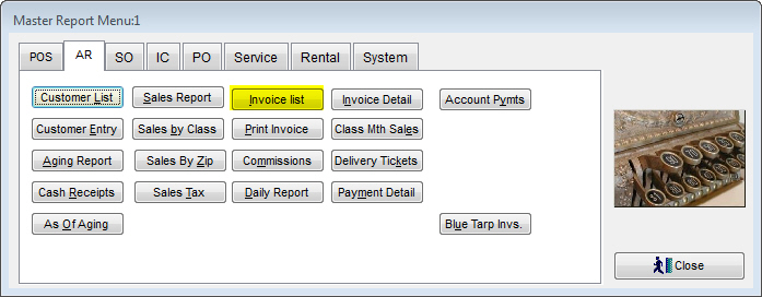
1. Go to AR | Reports and select Invoice list
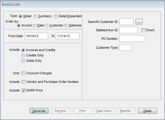
2. Leave the default values for the Type and Order by, but change the date range to the dates you are looking to reconcile with the sales statistics
3. Make sure to check the box to Include MSRP Price
4. Click on Generate
5. Once TransActPOS has generated the report, the Data View button is enabled. Click this to begin the export process.
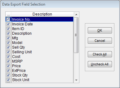
6. The Data Export Field Selection window will open. Click OK to export the data to the Data Viewer.
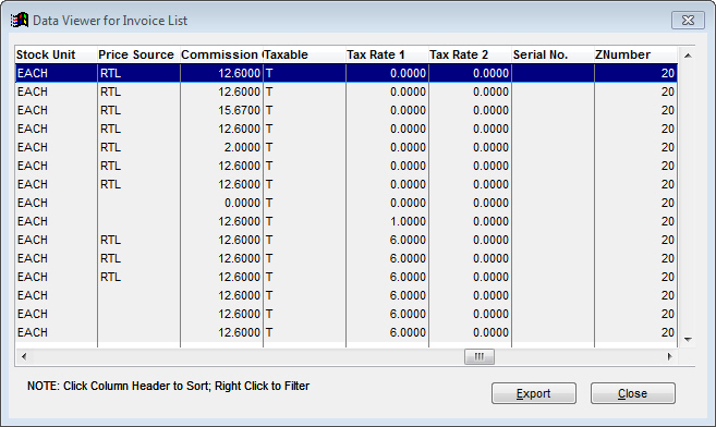
7. When the Data Viewer opens, scroll to the right and left click on the Tax Rate 1 column to order the data by tax rate. Once this is accomplished, click Export.
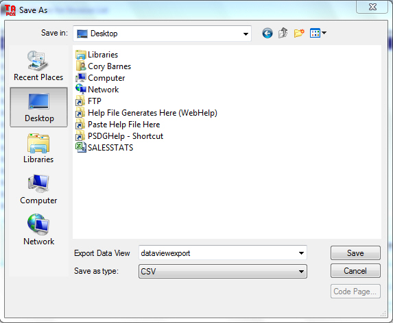
8. After clicking Export, the Save As window will appear. Select a folder on your workstation that you can easily access and change the file name to something that is easily identifiable.
9. After the file has been saved, minimize TransActPOS and locate the file you just created. Once you have found it, double left click it to open it in Excel.
It may be easier to separate the taxed and non-taxed items into 2 separate workbooks within Excel. If you wish to do this, proceed with step 10. If you wish to skip over this, go to step 17
10. Locate the change in the ntaxrate1 column (should be a change from 0 to a different rate)
11. Select the rows (left click hold on row numbers on the left side of the program and move the mouse down to the final row with data) after the rate change all the way to the bottom of the data
12. Press Ctrl + X to "cut" these rows
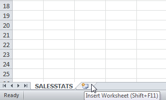
13. Select a new sheet by clicking the new sheet icon at the bottom of the page
14. In the new sheet, place your cursor (left click) in cell A2 and press Ctrl + V. This will "paste" the previously cut information into the cells.
15. Go back to the first worksheet and click the 1 on the left side (row 1) to select the entire first row. Press Ctrl + C to "copy" the information in row 1.
16. Go back into the second sheet and place your cursor in cell A1 and press Ctrl + V to paste the information.
Now the Excel document is separated into Non-Taxed (Sheet 1) and Taxed (Sheet 2) items
17. Along the top of the program, select Data.
18. Within each Sheet, press Ctrl + A to select all data on that worksheet. Once all information is selected, click Sort.
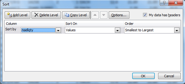
19. On the Sort screen, select nsellqty in the Sort by drop down menu. By default, the Order should be Smallest to Largest (which is what you need in this field). Click OK to sort the data.
20. In each worksheet, locate the last row that has a negative nsellqty and insert a row after it. To do this, right click on the row after the last negative value and click Insert.
21. Locate the yextprice column. In the newly created row, select the cell in this column and go to the Formula tab along the top.
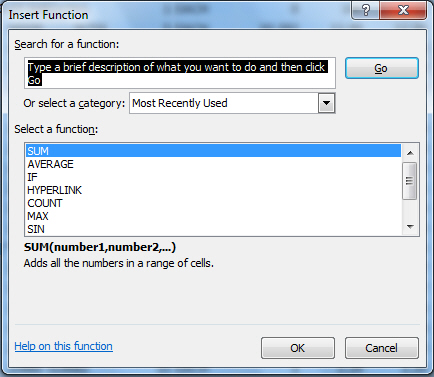
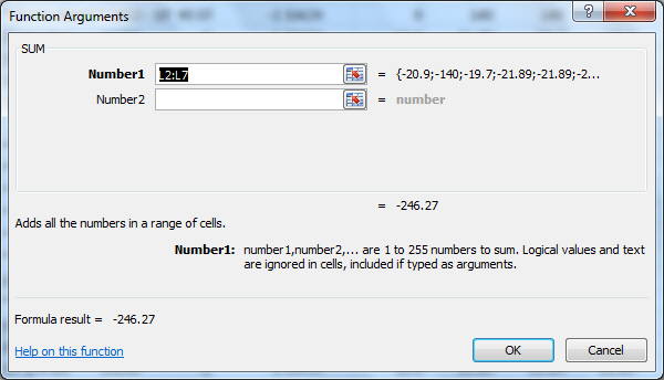
22. Click Insert Function to create an equation to figure out the total of all refunds. In the Insert Function screen, Sum should be the first one. If not, highlight it by left clicking it and click OK.
23. On the Function Arguments screen, the value entered in the Number1 field should be correct. Click OK to apply the function to this cell. You should now have the sum of all refunds in each sheet.
24. On each worksheet, insert 2 columns to the right of the yextprice column. To do this, right click on the column to the right of the yextprice column and click Insert. Do this twice and you will have two blank columns next to the yextprice column. These columns will be for finding the difference in MSRP and the price that the item was sold for.
25. Locate the first item after the sum of the refunds section and click the first new column for this item. In this column, we are determining what full retail should've been. To do this, enter the following equation into the field and press enter:
|
=G9*J9
(Column G is the nsellqty; Column J is the ylist; the number corresponds to the row you are currently in)
|
26. Once this equation is entered, you can save some time by left clicking the field we created in the previous step, pressing Ctrl + C to copy the equation, and press Ctrl + V in every cell below in this column to paste the equation for the given row.
27. Now, locate the first item as found in Step 25 and left click in the second new column. In this column, we are determining the difference between what was charged and what should have been charged. To do this, enter the following equation into the field and press enter:
|
=L9-M9
(Column L is yextprice; Column M is the first new column we created from step 25; the number corresponds to the row you are currently in)
|
28. Once the equation is entered, you can save some time like you did in step 26. Repeat step 26 for this column.
29. Now that we have the differences, we can do a sum of the difference column. To do this, click the empty cell right below the last difference (second new column you created) and click on Insert Function in the Formula tab (like you did in 21 and 22). Sum should be the first default function, but if not, select it and press OK. On the following screen, the information entered into the Number1 field should be correct. Click OK to add up the differences. This total should be your discounts for each tax category within pennies.